This tutorial explains how to do reverse vlookup in Excel. There is an Excel add-in that can do reverse lookup in the same manner that vLookup is done. It adds a new function to Excel (called rLookup), and you can use that function to do reverse vLookup, in the same manner as you do vLookup. It is very similar to the native VLOOKUP function of Excel.
In vLookup, Excel matches data in first column of the selected table, and then you can fetch corresponding value from any column of that table. What this reverse lookup function does is it matches data in the last column of the selected table, and then you can fetch values from any column of that table.
If you have used vLookup a few times, you know sometimes this limitation becomes a pain that data can only be looked up in the first column of the selected table. rLookup takes away that pain a bit by letting you lookup on the last column of the table.

If you have been following this website, you already know how to lookup multiple items in Excel, and how to highlight all search results in Excel. Now we will enhance your knowledge further by letting you know how to do reverse vLookup in Excel.
How to do Reverse Lookup in Excel?
If you know how to use the VLOOKUP function in excel, then it will not be very difficult to use this add-in. This add-in adds a function rlookup that takes the same arguments as vLookup, so you can start using it immediately. You can see the syntax for rLOOKUP function as shown below:
rLOOKUP (“LOOKUP VALUE“, TABLE, Column Number)
- LOOKUP VALUE: The value you want to look up.
- TABLE: The range of cells containing the data.
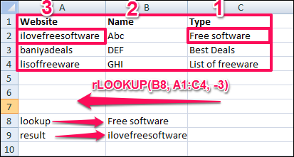
- COLUMN NUMBER: Position of the column from the lookup column in left to right direction. For reverse lookup, you will have to assign a negative number that indicates that the lookup will be performed in the reverse manner. See the example below.
rLOOKUP(“ilovefreesoftware”, A1:B6, -2):
It means that it will lookup for data in the last column of the selected table and will search for string “ilovefreesoftware” in that. Once the string is found, it will return data from 2nd column on the right.
rLOOKUP(“ilovefreesoftware”, A1:B6, 2):
This will be same as a normal vLookup function. It will search for data in the first column of the table, and will return result from the second column of that table.
Here are simple steps to use this function:
Step 1: Download and install rLOOKUP add-in from this link. After that it will integrate in the Excel until you remove it. And if you don’t know how to install an add-in in Excel then you may see here: link.
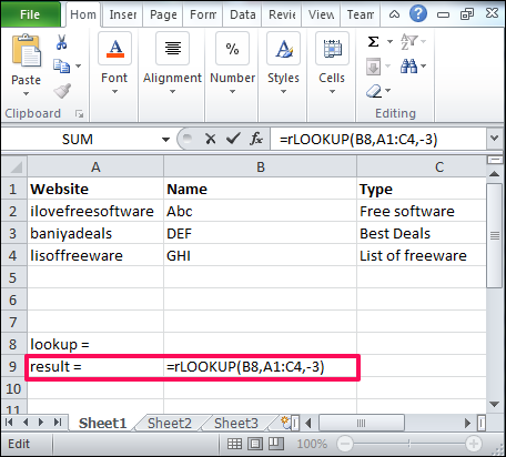
Step 2: Open a desired sheet that contains some data use the formula as I mentioned in syntax above. In my case I wanted to find out the name of the website using its type, so I put this formula in result cell: rLOOKUP(B8,A1:C4,-3)

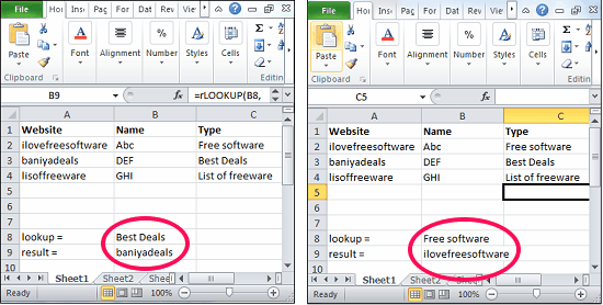
Step 3: Now, type different values in the lookup cell, you will see the corresponding result in the result cell. See the below screenshot.
In this way you can do reverse lookup in Excel using a very simple add-in.
Not only this add-in does what it promises, what I like most about this is that it also integrates the existing vLookup function, so the same rLookup function can be used for normal vLookup as well as reverse vLookup. All it needs is just removing a minus sign from the column index number.
Also see: How to Change case of text in Excel.
My Final Verdict
This plugin makes it amazingly easy to perform reverse vLookup in Excel. I have been using vLookup in Excel since years, and have always wondered why isn’t there an option to do a reverse Lookup. This plugin fills that gap. I really hope someday Microsoft decides to add this feature to the native vLookup itself.